Can machines hear an activity, not just a sound?
Large audio-language models recognise atomic events — a door slam, a keyboard click — with ease. This benchmark asks whether they can compose those events into the everyday human activities they imply.
Atomic recognition is solved. Abstraction is not.
Everyday actions — setting a table, cleaning a room, making coffee — are not single sounds. They emerge compositionally from sequences of temporally distributed, loosely-coupled acoustic cues. Recognising the constituent events is necessary but not sufficient.
Existing benchmarks reward identifying dog barking or glass breaking. They say little about whether a model can hear running water, then cupboard movement, then metallic clatter, and infer someone is preparing a meal. This benchmark isolates that second step.
Two probe families on a 2×2 difficulty ladder
The benchmark is organised around two probe families that ask fundamentally different questions: a flat family, which infers the activity directly, and a hierarchical family, which works down the taxonomy from coarse category to fine label. The five protocols are members of these two families, not a flat list — and the central result is that which family a protocol belongs to, more than its individual mechanics, determines whether decomposition helps or hurts. Every clip is also placed on two orthogonal axes of difficulty, grounded in CLAP embedding geometry; CLAP organises the data but is never itself evaluated.
Two difficulty axes
Central exemplars sit near the class prototype; peripheral ones are acoustically atypical instances of the same activity.
Distant distractor labels are acoustically far; near ones are confusable neighbours. Labels in a direct ancestor–descendant relationship with the target are excluded to prevent trivial taxonomic confounds.
Two probe families
Infer the activity in one step, with no taxonomic scaffolding.
Reason over the taxonomy, from coarse category down to fine label.
The two families behave oppositely under decomposition: within the flat family, grounding inference in explicit event recognition (P2) tends to hurt; within the hierarchical family, decomposing the prediction across taxonomy levels (H2) reliably helps. P2 is a single forward pass, not a chain-of-thought loop. Closed-set chance is 25% (four candidate labels); open-ended has no fixed baseline. Every model is evaluated zero-shot — flat closed-set protocols use 15 prompt templates, hierarchical use 5, open-ended uses 10.
Accuracy slides downhill — for every model family
Mean direct-prompting (P1) accuracy by model category, across the four splits. Toggle a family to compare slopes; the steeper the line, the more brittle the family is to acoustic ambiguity.
The full leaderboard, sortable
Top-1 accuracy on every split, for any of the five protocols across both probe families. Click a column to sort; cell shading tracks accuracy. The dropdown groups the flat family (P1 direct, P2 event-grounded, P3 open-ended) and the hierarchical family (H1 joint, H2 sequential) — switching within versus across families is where the interesting contrasts appear. Open-ended (P3) is evaluated only on the easiest and hardest splits, so its other cells read "—".
Cross-protocol explorer
Per-model accuracy on any protocol × split. The protocol dropdown spans both probe families (P1–P3 flat, H1–H2 hierarchical); bars are coloured by model family.
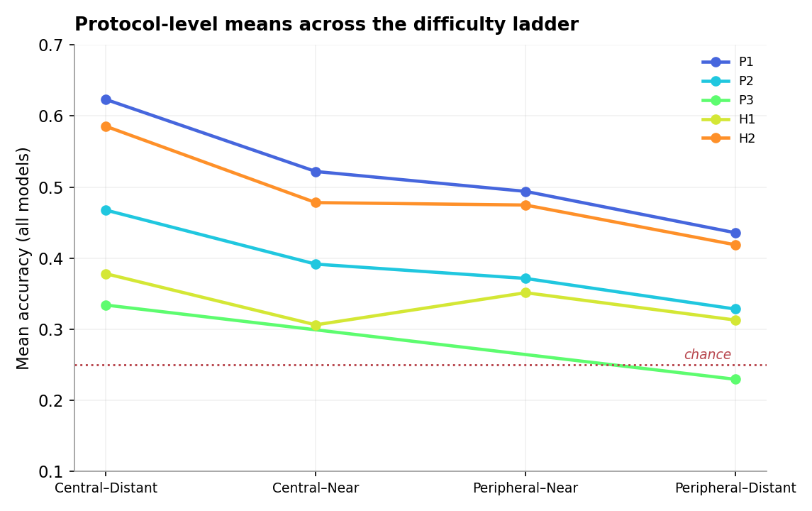
Protocol means across the ladder
Mean accuracy per protocol, averaged over all models across the difficulty ladder. Event grounding (P2) generally falls below direct inference (P1), while sequential hierarchical decomposition (H2) lifts fine-grained accuracy above the joint baseline (H1).
What the numbers say
The paper draws three consistent conclusions, and the sharpest of them is a contrast between the two probe families: decomposition is not uniformly good or bad — it depends entirely on which family does it. Within the flat family, grounding inference in explicit events (P2) hurts; within the hierarchical family, decomposing along the taxonomy (H2) reliably helps. Alongside this, typicality robustness is largely decoupled from overall capability, and under joint difficulty all model families converge near chance. The findings below track those conclusions, with supporting numbers recomputed from the reported tables.
Typicality robustness is decoupled from capability. Holding distractors fixed, moving from central to peripheral exemplars costs ~11 points on average; moving to near distractors costs ~10 points. Most models fall below the C-Dist↔P-Near diagonal, and the degradation is largely independent of overall accuracy — Qwen3-Omni Captioner is strongest on the easiest split yet drops sharply (Δ≈−0.34), while Gemini-2.5-Flash-Lite is nearly invariant (Δ≈−0.02). Robustness should be treated as its own evaluation axis, not a byproduct of capability.
The two stressors partly overlap rather than compound. The combined easy→hardest drop (mean ≈ 17 points) is smaller than the sum of the two single-axis drops (≈ 21 points): for 26 of 27 models the joint effect is sub-additive. A model already hurt by atypical input has less left to lose to near distractors.
In the flat family, event grounding is a near-universal penalty. Within Probe Family I, decomposing direct inference into explicit event recognition followed by activity inference (P1→P2) consistently regresses across model families and difficulty levels — almost every model lands below the diagonal at both the easiest and hardest splits. Inside the flat family the extra prediction step imposes a uniform processing cost rather than amplifying model strengths.
In the hierarchical family, sequential decomposition reliably helps. Within Probe Family II — and in sharp contrast to the flat family — conditioning fine-grained prediction on a predicted coarse category (H1→H2) improves fine accuracy for 25 of 26 models at each split. Decomposition that contracts the hypothesis space along the taxonomy reduces effective search complexity without adding failure modes. The two families thus draw opposite conclusions about decomposition: it is the family, not decomposition per se, that decides the outcome.
Test-time reasoning helps in proportion to how much intermediate abstraction the protocol needs. Across families with thinking / no-thinking variants the gain is protocol-dependent: minimal on direct inference (P1, Δ≈+0.03), substantial on event-grounded inference (P2, Δ≈+0.12), and intermediate on hierarchical abstraction (H1/H2, Δ≈+0.05). Thinking is a remedy for ambiguity and multi-step structure, not a free boost for direct retrieval.
Joint difficulty erodes between-class separability. At the easiest split, Frontier and Reasoning models reach ≈0.60 accuracy while Open-Source models cluster near 0.41. That separation collapses with difficulty, converging to a narrow 0.40–0.48 band at Peripheral–Near — only marginally above chance. Compositional auditory understanding is a distinct capability not yet reliably acquired by current models.
Hierarchical: joint vs. sequential
Fine-grained accuracy under joint single-turn prediction (H1) vs. sequential multi-turn decomposition (H2), across the difficulty ladder. H2 lifts fine accuracy above H1 at every split — taxonomy-aligned decomposition reliably helps.
Direct (P1) vs. event-grounded (P2)
Each point is a model. Above the diagonal ⇒ event grounding helps; below ⇒ it hurts. Nearly all models sit below the line at both splits.
Central–Distant (easy)
Peripheral–Near (hard)
Which activities are hard — and what they get confused with
Per-class top-1 accuracy for the strongest model in each family, on the easiest and hardest splits. Each row is a SALT label; markers show where the four models land. Labels are ordered by mean accuracy, so the acoustically hardest routines sink to the bottom.
Per-class accuracy ridgeline
Circle = Central–Distant (easiest), cross = Peripheral–Near (hardest). The grey band behind each row is that class's CLAP embedding spread (±1σ of the prototype) — a proxy for how acoustically diffuse the class is.
Coarse-group confusion
Where predictions land when the true activity is cooking, cleaning, or organising — the acoustically overlapping routines the paper flags. Rows are normalised; the diagonal is correct attribution. Click to open a larger view.
Hardest and easiest classes
Mean accuracy across the four models and both splits, ranked.
Explore the taxonomy
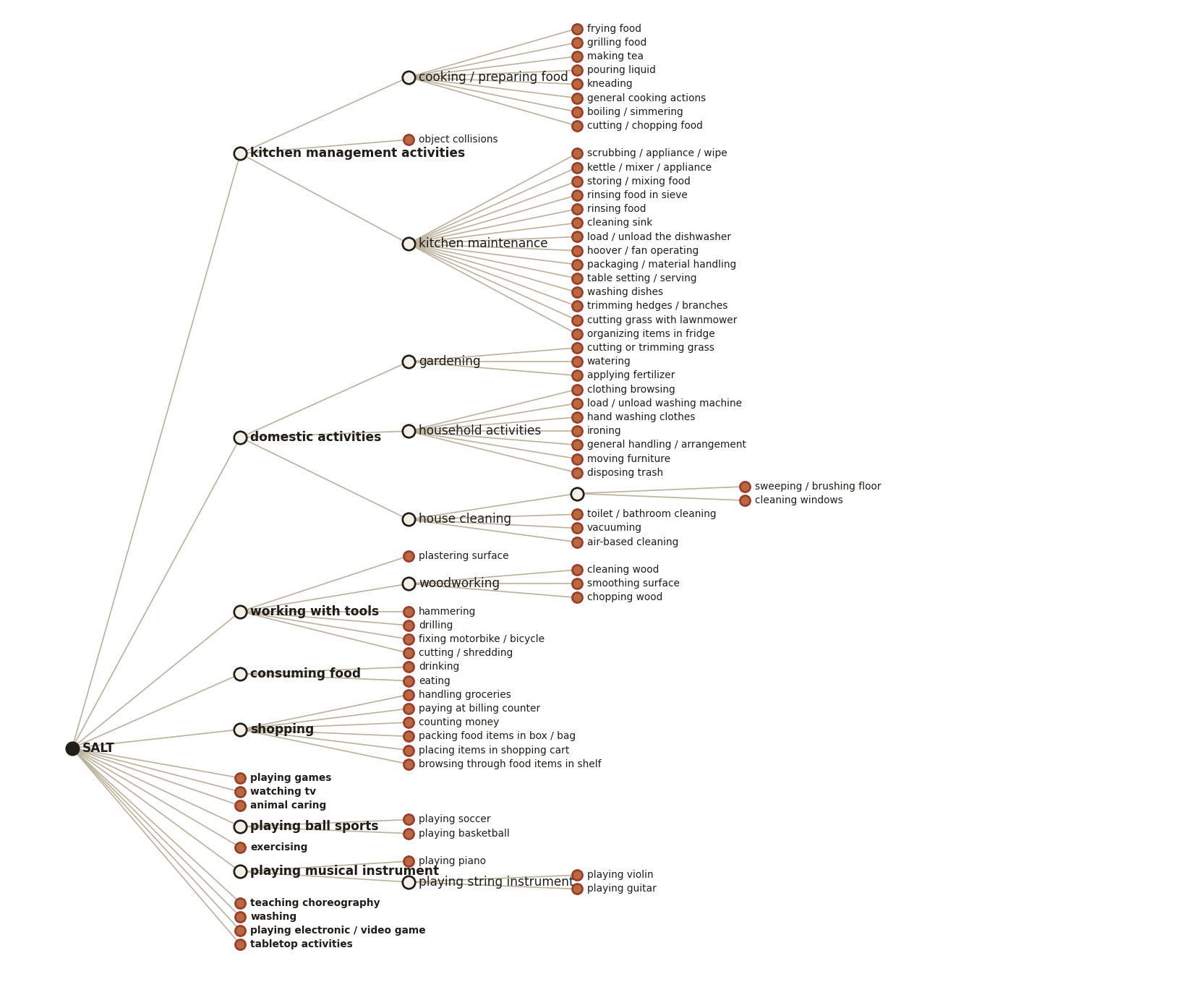
A hierarchy of audio-identifiable human activities. Click any node to expand or collapse its children. Solid dark nodes hide collapsed subtrees; clay-coloured nodes are leaves. The interactive tree shows the audio-bearing subset; the full taxonomy spans 99 nodes across up to five levels. Click the background (or the ⤢ corner icon) to open a larger interactive view.
Pipeline at a glance
5–10 second segments
Naturalistic recordings are cut into 5–10s single-label segments — enough context for activity-level inference, short enough to compare across fixed-input models. Each segment keeps its original activity label.
CLAP prototypes
Each class gets a centroid prototype. Central exemplars lie nearest it; peripheral ones farthest. CLAP is an organiser only — it is never scored.
Two families, five protocols
A flat family (direct, event-grounded, open-ended) and a hierarchical family (joint, sequential), each with controlled distractors drawn by embedding distance.
All figures and statistics on this page are derived solely from the values reported in the submission's tables; no raw model outputs or identifying metadata are included.
The prompts behind every number
Each template is shown exactly as issued to the model, with its output-format rules appended at the end (both turns, for the multi-turn probe). Templates are reproduced verbatim; only HTML escaping has been applied.